The problem
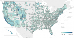
In the previous blog post, I tried to rank cities of United States based on the different type of data, Zillow housing prices, for instance, to find my next home. During the effort, I realized that Zillow dataset only contains 48% of the counties in the United State. To put my machine learning skills in practice I thought it's a good idea to predict the prices for the missing counties.
Data preparation, preprocessing, and exploration
The Kaggle dataset has around 60 features for 3510 counties, so it's worth trying to build the predictive model based on the combination of the Kaggle dataset and available housing prices of Zillow dataset, and use it to predict the missing housing prices. So, I joined the datasets based on county name. Then normalized the dataset using the min-max method to make sure regardless of the prediction method that I use I'll get a relevant result. To have a better understanding of the data, here are some diagrams, drawn using Seaborn package.
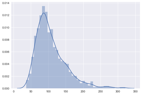
(I cut the long tail at 4th StdDev)

At the first attempt, I used scikit-learn's RFECV function and linear regression as the predictor to first, estimated the level of the complexity of the required model. Second to check if feature selection could be an option to reduce the dimensionality of the dataset.
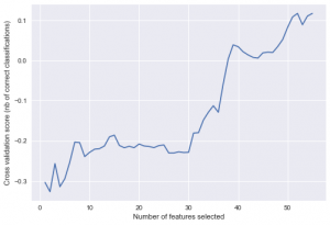
As far as the diagram shows the model benefits from a higher number of features so it's a better idea to keep all the features. the best-achieved score the trained model is R^2 = 0.12 which is a very low score. As the result, we need a more complex method than linear regression to handle the complexity of our dataset.
Building the predictor
I'm a fan of ensembling methods especially Random Forest. That being said, I also tried other methods such as Linear Regression, Decision Tree, and SVR but RF has the best performance.
To find best hyperparameters of the RF model I used GridSearchCV and RandomForestRegressor to utilize Exhaustive Grid Search. After some trial and error, I decided to run the Grid search to tune "depth of the tree" in the range of 20 to 50 and "threshold for the impurity of nodes" in the range of 1e-8 to 1e-7. To save some time I considered 5 for the number of Cross Validations. My initial test shows that 100 estimators seemed enough for the training of Random Forest.
param_grid = [{
        'max_depth':np.arange(20,50,10),
        'min_impurity_split':np.linspace(1e-8,1e-7, num=5)

        }]
estimator_g = GridSearchCV(RandomForestRegressor(n_estimators=100, random_state=123),
                         param_grid = param_grid,
                         cv = 5
                         )
estimator_g.fit(X,Y)
result_df = pd.DataFrame(estimator_g.cv_results_)
The following table shows top 10 combinations out of 30:
| parameters | mean_validation_score |
|---|---|
| {'max_depth': 30, 'min_impurity_split': 8.9999999999999999e-08} | 0.480304891 |
| {'max_depth': 40, 'min_impurity_split': 8.9999999999999999e-08} | 0.480103623 |
| {'max_depth': 30, 'min_impurity_split': 7.0000000000000005e-08} | 0.480070149 |
| {'max_depth': 40, 'min_impurity_split': 7.0000000000000005e-08} | 0.479873108 |
| {'max_depth': 30, 'min_impurity_split': 8.0000000000000002e-08} | 0.479230345 |
| {'max_depth': 40, 'min_impurity_split': 8.0000000000000002e-08} | 0.479087128 |
| {'max_depth': 30, 'min_impurity_split': 5.9999999999999995e-08} | 0.479059378 |
| {'max_depth': 40, 'min_impurity_split': 5.9999999999999995e-08} | 0.478921322 |
| {'max_depth': 30, 'min_impurity_split': 9.9999999999999995e-08} | 0.478321218 |
| {'max_depth': 30, 'min_impurity_split': 4.9999999999999998e-08} | 0.478092421 |
Having R^2 as the validation score is not promissing but for now it's the best result I could achive with this dataset and estimator. More on this in the "Evaluating the model" section.
Next, we need to train the model with the labeled data that we have to build the RF model:
estimator = RandomForestRegressor(
        n_jobs=3,
        max_depth=30,
        min_impurity_split=8.9999999999999999e-08,
        random_state=123,
        n_estimators=100
       )
Evaluating the Model
I usually use learning curve to evaluate the generalization of the model, in other words, to see if the model is underfitting or overfitting. The learning_curve function makes the evaluation easy by determining the training and test scores for different sizes of the training set.
estimator = RandomForestRegressor(

        max_depth=30,
        min_impurity_split=8.9999999999999999e-08,
        random_state=123,
        n_estimators=100
        )

# to illustrate the results
train_sizes, train_scores, test_scores =\
    learning_curve(estimator=estimator, X=X, y=Y,
                   train_sizes=np.linspace(0.1, 1.0, 10),
                   scoring='r2',
                   cv=5,
                   n_jobs=3)
train_mean = np.mean(train_scores, axis=1)
train_std = np.std(train_scores, axis=1)
test_mean = np.mean(test_scores, axis=1)
test_std = np.std(test_scores, axis=1)

plt.plot(train_sizes, train_mean,
         color='blue', marker='o',
         markersize=5,
         label='training score')
plt.fill_between(train_sizes,
                 train_mean + train_std,
                 train_mean - train_std,
                 alpha=0.15, color='blue')
plt.plot(train_sizes, test_mean,
         color='green', linestyle='--',
         marker='s', markersize=5,
         label='validation score')
plt.fill_between(train_sizes,
                 test_mean + test_std,
                 test_mean - test_std,
                 alpha=0.15, color='green')
plt.grid()
plt.xlabel('Number of training samples')
plt.ylabel('R^2')
plt.legend(loc='lower right')
plt.ylim([-1.0, 1.0])
plt.show()
This diagram is the result of the above code:
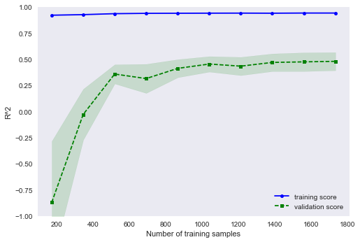 The gap between training score and validation score indicates that the model suffers from high-variance. So far I've tried out-of-bag sampling or reducing the number of features but I couldn't fix this over-fitting problem. Speaking of features let's take a look at the top 5 features ranked by our trained RF model:
- Building_permits_2014 (0.171863)
- state_politic (0.140187)
- Accommodation_and_food_services_sales_2007__1_000_ (0.100334)
- Population_percent_change__April_1_2010_to_July_1_2014 (0.047493)
- Persons_below_poverty_level_percent_2009_2013 (0.034397)
Seeing demographic related features, such as number 4 and 5, in the list is not surprising but I personally surprised seeing state politics as the second rank.
Predicting missing data
Our model is not perfect but that doesn't stop us from using it for predicting the missing housing prices. As we have a trained model ready the prediction part is easy we just need to call the "fit" function. Here is the distribution of the predicted values:
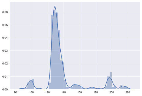
At first, I thought something is wrong with this distribution but after some research, I stand corrected. The matter of fact is that the missing values in the Zillow dataset (or any other dataset) do not necessarily follow the distribution of the dataset.
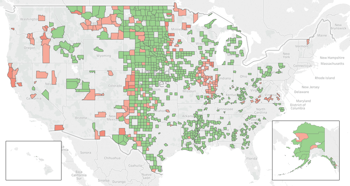
Let's call it a day for now and use our model to complete the coverage map:

Conclusion
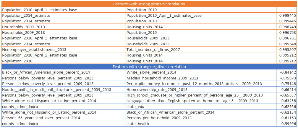
I believe to achieve a better result I need to put together a reference dataset, like the one I took from Kaggle, with more up-to-date and relevant features. As we saw in the correlation result, although the dataset has more than 60 features, we have too many features with strong correlation basically because there are demographic data. I still don't have any use for the predicted data but it was a pleasant experience using scikit-learn, I enjoyed the ease of use and clarity of the documentation. Look forward to use it in next projects.