


Introduction
Brake test is a time consuming and costly operation for the factories. The plant needs to shut down the robots to perform the test. It worth exploring to see if it is possible to predict the test results based on historical data. At the time of this writing, we approach this problem as a binary classification problem.
Data Preprocessing
The receiving data needs to be cleaned and wrangled to be ready to be fed to a machine learning model. In this section, the necessary steps are explained.
Feature Engineering
Brake test data is in the form of a time series as it records several features for each robot during the brake test over time. There are limited tools and methods suitable for working with time series so that would be helpful if we could transform the problem to classification problem which is easier to solve. To do that, a moving window can be used. For example, averaging `torque_peak` for the past 5 days (excluding the current day) and assign it to a variable in the current day, see the table below for more clarity. Please note we do that for each axis and individual robots separately, so in the below example, all other axis and robots are not being shown.
| row no. | torque_peak | torque_peak_avg_5 | axis_test_date | robot_serial | axis_number |
| 1 | 19.0936 | Avg of row 2 to 7 | 2017-04-27 | 737411 | 1 |
| 2 | 19.0939 | Avg of row 3 to 8 | 2017-04-26 | 737411 | 1 |
| 3 | 19.0877 | Avg of row 4 to 9 | 2017-04-25 | 737411 | 1 |
| 4 | 19.0981 | Avg of row 5 to 10 | 2017-04-24 | 737411 | 1 |
| 5 | 19.0932 | … | 2017-04-23 | 737411 | 1 |
| 6 | 19.0888 | … | 2017-04-22 | 737411 | 1 |
| 7 | … | … | … | … | … |
| 8 | … | … | … | … | … |
| 9 | … | … | … | … | … |
| 10 | … | … | … | … | … |
The following metrics were calculated:Average, Standard Deviation, and Correlation (of the variable and timestamp) for all variables of interest for a 3-day and 5-day time window: [‘avgMotTemp’, ‘observed_brake_torque’, ‘observed_static_friction’, ‘torque_const_move’, ‘torque_limit_cmd’, ‘torque_peak’] => [‘avgMotTemp_avg_5’, ‘avgMotTemp_stddev_5’, ‘avgMotTemp_corr_5’, ‘observed_brake_torque_avg_5’, …]. We add an additional 3-day time window because we have a few robots with an available 5-day time window.
Another variable that was added is `test_timestamp` which basically is the result of `axis_test_date` to seconds.
Output variables
Dealing with binary class output variables is easier and more efficient than working with multiclass ones. Furthermore, labels other than `BT_BRAKE_TORQUE_OK` and `BT_BRAKE_NOT_OK` are so rare. So we decided to fold other labels into these two.
| Old overall_test_result | New | Count |
| BT_BRAKE_TORQUE_OK | BT_BRAKE_TORQUE_OK | 1747454 |
| BT_HOLDING_TORQUE_OK | BT_BRAKE_TORQUE_OK | 653 |
| BT_BRAKE_NOT_OK | BT_BRAKE_NOT_OK | 2218 |
| BT_BRAKE_TORQUE_LOW | BT_BRAKE_NOT_OK | 629 |
| BT_INCOMPLETE | removed | 15 |
| BT_MOTION_FAULT | removed | 1 |
Imputation
An n-day time window could result in Null values if the rows in the window are less than n. Furthermore, the Corr function could produce Null if one of the variables has zero variance. As a result, we need to impute the Null values:
- Considering 3-day time window instead of a 5-day time window as most of the robots have no data for 5 consecutive days
- Fill N/A using mean with the same Robot Type and overall_test_result
- Then fill N/A using mean with the just same overall_test_resut
- Then drop rows with N/A values as Scikit learn can’t handle N/As
- Remove all the robots without any recorded failure to make the dataset more balance
Here is the result:
| overall_test_result | Count | Ratio |
| BT_BRAKE_NOT_OK | 2781 | 0.0060005178 |
| BT_BRAKE_TORQUE_OK | 460679 | 0.9939994822 |
Analytics
Predicting brake test is a classification problem and because only %0.6 of observations are related to brake failure we are dealing with a highly imbalanced dataset. Base on my initial investigations Random Forest looks like a good choice for this problem for the following reason:
- It’s highly parallelizable in compare to Boosting based models
- In Scikit Learn the Random Forest function has a large set of parameters including the ones to deal with imbalanced datasets
Note: As mentioned before, the dataset is highly imbalanced as less than 0.1% of the observations are labeled ‘BT_BRAKE_NOT_OK’ so it makes sense to use some advanced methods such as undersampling ‘BT_BRAKE_TORQUE_OK’. Spoiler alert: It turned out the Random Forest can manage an imbalanced dataset even without using any balancing technic. - The ensembling nature of RF reduce the possibility of overfitting
Why undersampling methods would not work
With only around 2000 failed brake tests, undersampling provide us a too small dataset to train a model with. Some of my colleagues did try undersampling and got a great F1-score of 0.92 but there is a major flaw in their approach. They test the model with undersampled data which is wrong because do not represent real-world data. I reproduced their work and got a high F1-score of 0.96 but after testing it with the imbalanced test dataset, the F1-score dropped to 0.2.

The main reason for this phenomenon is that even if the model misclassifies %0.5 of the passed tests to fail, the Precision score falls below 0.5 and result in a low F1-Score.
Even more complicated methods such as Instance Hardness Threshold do not do better.
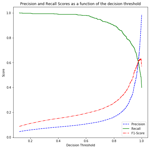
Trying oversampling methods
Oversampling means generating more observations of the minority class. Just duplicating current observation will not work so we need to use more advanced methods such as the Synthetic Minority Oversampling Technique (SMOTE) [CBHK2002] and the Adaptive Synthetic (ADASYN) [HBGL2008]. All of which perform perfectly on 5-fold cross-validation but poorly on unseen imbalanced data. Here is the Recall-Precision threshold for a Random Forest model fitted the oversampled data by ADASYC. Applying SMOTE results in a similar performance.
Leveraging Ensemble Learning
The Scikit-learn RandomForest supports three types of weighted sampling: ‘balanced’, ‘balanced subsample’, and No weight assignment. We will see if these methods help us to build a better prediction model.
I tried a randomized hyperparameter grid search to have an idea of the range of hyperparameters values.
# Number of trees in random forest
n_estimators = [int(x) for x in np.linspace(start = 100, stop = 600, num = 10)]
# Number of features to consider at every split
max_features = ['sqrt', 'log2', None]
# Maximum number of levels in tree
max_depth = [50, 100]
max_depth.append(None)
# Minimum number of samples required to split a node
min_samples_split = [10, 20, 40, 80]
# Minimum number of samples required at each leaf node
min_samples_leaf = [1, 2, 4, 8]
# Method of selecting samples for training each tree
bootstrap = [True, False]
criterion = ['gini']
class_weight=['balanced','balanced_subsample', None]
This is how the best performing model trained with all the features looks like:
Model with rank: 1
Mean validation score: 0.734 (std: 0.010)
Parameters: {'random_state': 42, 'n_estimators': 100, 'min_samples_split': 80, 'min_samples_leaf': 2, 'max_features': 'sqrt', 'max_depth': 50, 'criterion': 'gini', 'class_weight': None, 'bootstrap': False}

Model with rank: 2
Mean validation score: 0.734 (std: 0.013)
Parameters: {'random_state': 42, 'n_estimators': 377, 'min_samples_split': 40, 'min_samples_leaf': 1, 'max_features': 'sqrt', 'max_depth': 100, 'criterion': 'gini', 'class_weight': None, 'bootstrap': True}

Model with rank: 3
Mean validation score: 0.715 (std: 0.015)
Parameters: {'random_state': 42, 'n_estimators': 211, 'min_samples_split': 10, 'min_samples_leaf': 1, 'max_features': 'log2', 'max_depth': None, 'criterion': 'gini', 'class_weight': None, 'bootstrap': False}
The performance of the model is shown in the form of a learning curve diagram. It helps us check the bias-variance tradeoff and check the progress of the model. The current diagram shows that we cannot do much better with the current model and data.

Interestingly “class_weight” is None in the top 3 best performing model. So, the best model is achieved when we ignore the imbalance problem altogether.
Feature Importance
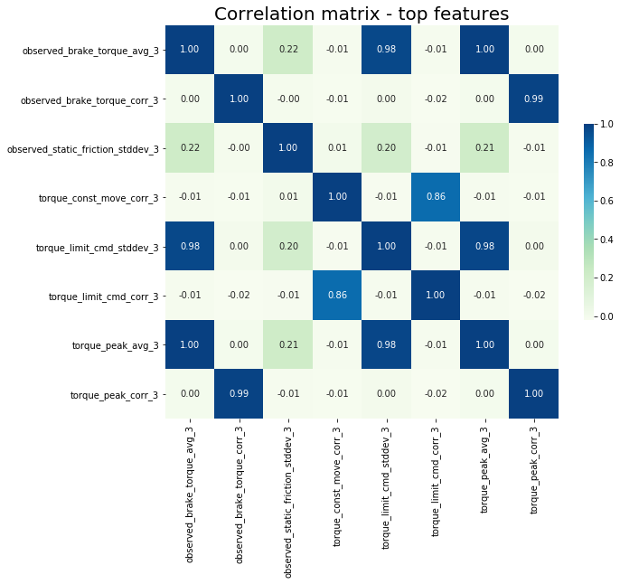
Before talking about feature selection it could be interesting to look at the correlation matrix (for a 3-day time window) to see if variables are correlated or not:
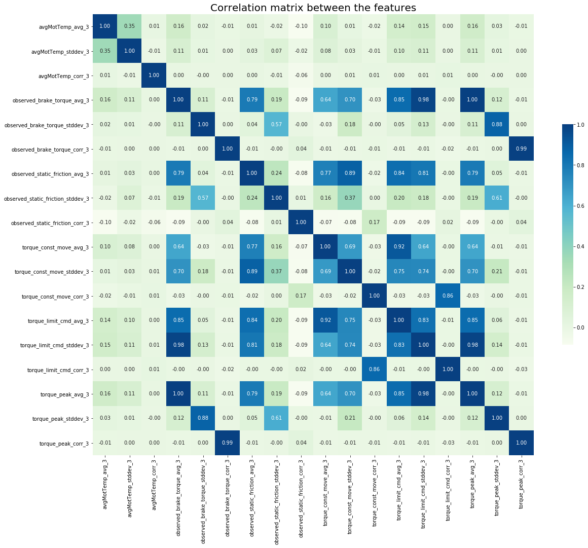
Using the sk-learn “SelectFromModel” function we can find the most important feature in which their score is the above median of all scores. Please bear in mind that because of the random nature of ensemble methods the order of the list is not deterministic. I also ran this for the combination of 3-day and 5-day time window but as expected the first 5-day feature (‘observed_static_friction_stddev_5’) appears at the 16th place. Here the correlation matrix of top features for a 3-day time window.
Note: “torque_limit_cmd_stddev_3” added later based on a model with a 0.3 threshold. See the Threshold Tuning section.
Fit the model to the data with selected features
I used the same hyperparameter grid as before to narrow the exhaustive search space, here are the top results:
Model with rank: 1
Mean validation score: 0.744 (std: 0.010)
Parameters: {'random_state': 42, 'n_estimators': 377, 'min_samples_split': 40, 'min_samples_leaf': 1, 'max_features': 'sqrt', 'max_depth': 100, 'criterion': 'gini', 'class_weight': None, 'bootstrap': True}

Model with rank: 2
Mean validation score: 0.743 (std: 0.013)
Parameters: {'random_state': 42, 'n_estimators': 100, 'min_samples_split': 80, 'min_samples_leaf': 2, 'max_features': 'sqrt', 'max_depth': 50, 'criterion': 'gini', 'class_weight': None, 'bootstrap': False}

Model with rank: 3
Mean validation score: 0.719 (std: 0.014)
Parameters: {'random_state': 42, 'n_estimators': 211, 'min_samples_split': 10, 'min_samples_leaf': 1, 'max_features': 'log2', 'max_depth': None, 'criterion': 'gini', 'class_weight': None, 'bootstrap': False}
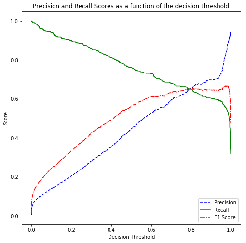
And the learning curve for the top-performing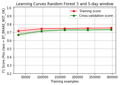 model. We improved the result slightly:
Threshold tuning
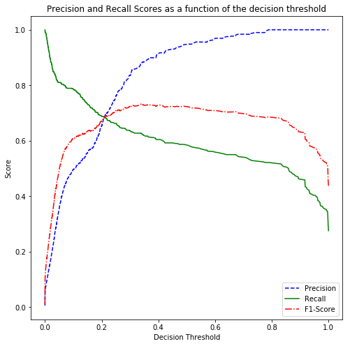
Considering that “class_weight” remained None in the top model performers, it is worth checking if changing the decision threshold improves the results. Here is the Precision-Recall curve:
Normally, in binary class datasets, sk-learn considers 0.5 as the threshold to decide which class to choose. The above shows that the 0.5 threshold results in low Recall. Move the threshold to 0.3 to help us achieve the highest F1 score possible.
By using the original hyperparameter grid and apply the 0.3 thresholds, the F score increased to 0.751
Model with rank: 1
Mean validation score: 0.751 (std: 0.015)
Parameters: {'random_state': 42, 'n_estimators': 400, 'min_samples_split': 40, 'min_samples_leaf': 4, 'max_features': 'sqrt', 'max_depth': None, 'criterion': 'gini', 'class_weight': None, 'bootstrap': True}

Model with rank: 2
Mean validation score: 0.750 (std: 0.014)
Parameters: {'random_state': 42, 'n_estimators': 366, 'min_samples_split': 40, 'min_samples_leaf': 2, 'max_features': 'sqrt', 'max_depth': None, 'criterion': 'gini', 'class_weight': None, 'bootstrap': True}

Model with rank: 3
Mean validation score: 0.750 (std: 0.016)
Parameters: {'random_state': 42, 'n_estimators': 100, 'min_samples_split': 80, 'min_samples_leaf': 1, 'max_features': 'sqrt', 'max_depth': 100, 'criterion': 'gini', 'class_weight': None, 'bootstrap': True}
Exhaustive Hyperparameter search
After finding out the important features, general values of hyperparameters, and the decision threshold, now it’s time to use an exhaustive search:
Expand source
{'n_estimators': [395, 400, 410],
               'criterion': ['gini'],
               'max_features': ['sqrt'],
               'max_depth': [50, None],
               'class_weight' : [None],
               'min_samples_split': [37,38, 39],
               'min_samples_leaf':[2,3],
               'bootstrap': [True],
                'random_state': [42],
              'n_jobs' : [10]}
results:
Model with rank: 1
Mean validation score: 0.754 (std: 0.016)
Parameters: {'bootstrap': True, 'class_weight': None, 'criterion': 'gini', 'max_depth': 50, 'max_features': 'sqrt', 'min_samples_leaf': 3, 'min_samples_split': 38, 'n_estimators': 400, 'n_jobs': 10, 'random_state': 42}

Model with rank: 1
Mean validation score: 0.754 (std: 0.016)
Parameters: {'bootstrap': True, 'class_weight': None, 'criterion': 'gini', 'max_depth': None, 'max_features': 'sqrt', 'min_samples_leaf': 3, 'min_samples_split': 38, 'n_estimators': 400, 'n_jobs': 10, 'random_state': 42}

Model with rank: 3
Mean validation score: 0.753 (std: 0.016)
Parameters: {'bootstrap': True, 'class_weight': None, 'criterion': 'gini', 'max_depth': 50, 'max_features': 'sqrt', 'min_samples_leaf': 3, 'min_samples_split': 38, 'n_estimators': 410, 'n_jobs': 10, 'random_state': 42}
Conclusion
Despite all our effort, we could not reach F1-Score above 0.76. I believe that’s because of the following reasons:
- The data do not cover robots and dates consistently. That results in a low learning rate as the model does not have enough data for a given robot to find the patterns.
- Too many brake tests with inconsistent results are being run on each robot per day. That makes building a classification model harder.
- The low rate of brake test failure result is a highly imbalanced dataset which is hard to approach with common methods.
What to do next?
The possible solutions to the mentioned problems could be:
- Trying to clean data by applying more domain knowledge. i.e. removing or merging multiple test results per day per robot into one observation
- Acquiring more consistent brake tests from manufactures
- Extracting more variables/information from the brake test logs currently we use “[‘avgMotTemp’, ‘observed_brake_torque’, ‘observed_static_friction’, ‘torque_const_move’, ‘torque_limit_cmd’, ‘torque_peak’]”, there are as many more.
- Trying new ways to deal with the time series problem other than folding it by aggregate functions. e.g. Recurrent Neural Networks